 Cassette Split Systems
 Safety Gloves
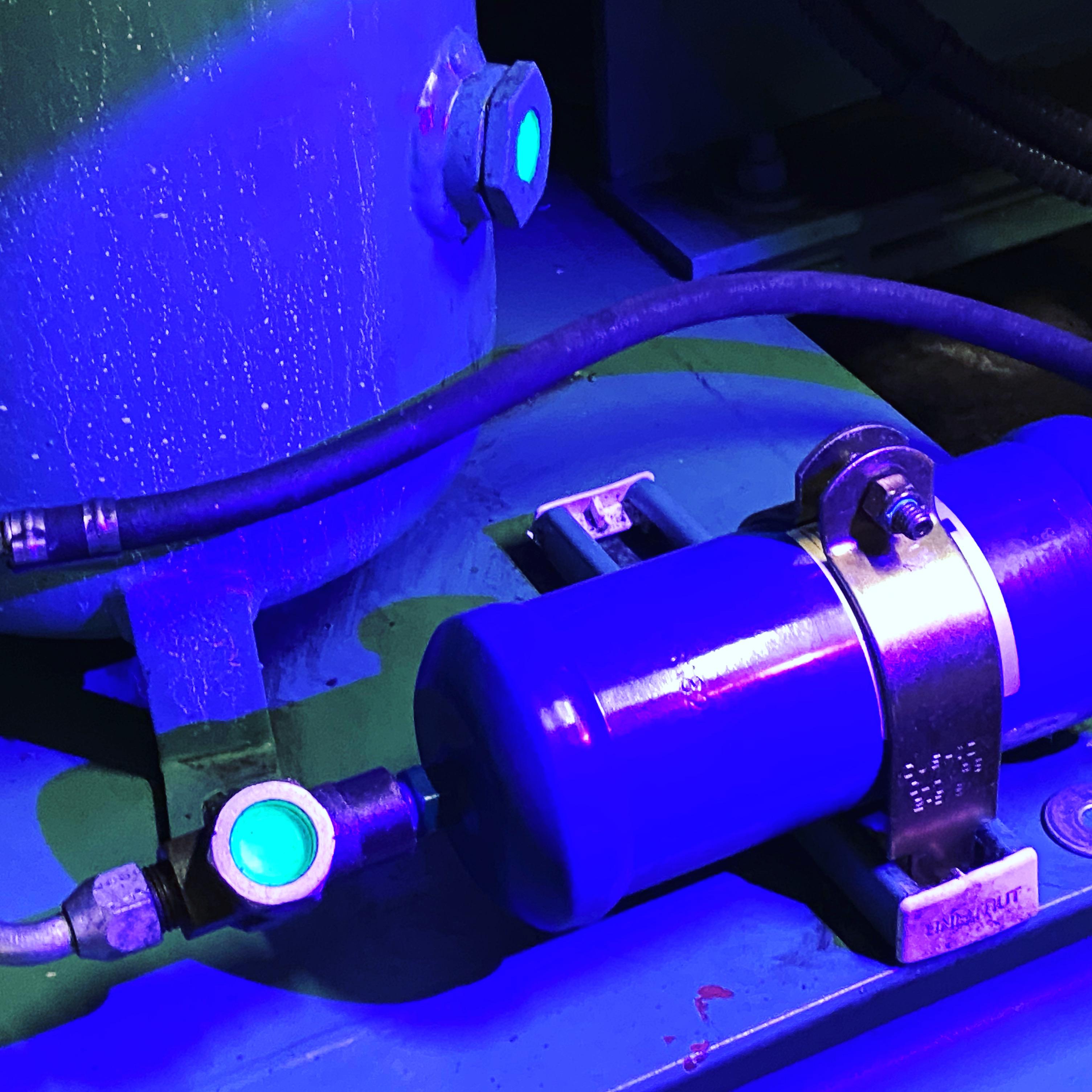 UV Leak Detection
 Condensate Drain Pipe
 Nitrogen Regulators
 Filter Driers
 Filter Cores for Core Shells
MASTERCLASS – AIR CONDITIONING TECHNOLOGY
Volume 37 – Cooling Mediums
In the previous two articles, a method for establishing the condition and volume of air that had to be cooled by the evaporator in order to remove excess heat from the conditioned space was examined. In addition the various options for circulating air were covered.
We will continue with the theme of conveying the cooling medium, air, to and from the conditioned space by the use of ducting.
___________________________________________________________________
As with many aspects of engineering, particularly refrigeration and air conditioning, we are faced with a number of compromises that must be resolved before we can start to design the ducted system.
Having calculated the cooling load, it is important to establish the primary design considerations with the client. The parameters we should consider and resolve are;
- How critical are the resulting noise levels? If the level of noise is crucial to the installation then we need to limit the velocities within the ductwork which then in turn determines the sizes of ducting.
- If the capital cost of the project is the primary consideration, over and above noise or running cost, then duct size and shape become the controlling design factors.
- Where running cost is the primary consideration then duct size, shape and velocity will influence the design.
- The last aspect that has to be considered is the space available for the ductwork. The space may also determine duct shape and is also likely to affect the duct velocities.
Once the above parameters have been considered, we have the option of two types of system and four methods of calculation.
Systems are defined as Low Velocity (Low pressure) with operating velocities up to 10 m/s, Medium Velocity (Medium Pressure) 10 to 20 m/s and High Velocity (High Pressure) which use velocities between 20 to 40 m/s.
High velocity systems tend to be used on very large projects where the increased cost of noise reduction and fan power are offset by the reduction in duct dimensions and duct space with their associated costs.
Low velocity systems are used in the majority of installations. The low pressures used allow light weight duct construction, lower fan power, higher air leakage rates and lower noise levels that can dispense with the use of noise silencers.
The calculation method is usually determined by the size and complexity of the project, this is because the gains in efficiency resulting from the greater accuracy of the more sophisticated calculation are too small to measure on a single room or small shop installation.
The methods of calculation are velocity reduction, equal friction, static regain and constant velocity.
Equivalent rectangular dimensions:
Generally when designing a ducted system the required cross sectional areas are defined by the required velocity. This area is based on circular duct dimensions but if rectangular ducts are to be used then the equivalent dimensions have to be calculated.
The equivalent rectangular dimensions take into consideration the aspect ratio of the duct i.e. The longest side divided by the shorter side e.g. a rectangular duct having sides of 400 mm x 200 mm = 400/200 = aspect ratio of 2:1. This duct has a cross sectional area of 0.08 m2. However you could have a duct of 75 mm x 1067 mm which gives the same area but its characteristics will be significantly different to the first duct. The 400 mm x 200 mm duct has a surface area of 1.2 m² per lineal metre length while the 75 mm x 1067 mm duct has a surface area of 2.284 m² per metre and since duct resistance is a function of velocity and surface friction, it follows that a duct with a high aspect ratio will have a higher resistance than a duct with a low aspect ratio. Therefore a duct which is square in section will have an aspect ratio of 1:1 and apart from a circular duct of the same area, will have the lowest internal surface area and the lowest friction.
To calculate the equivalent diameter (or more correctly the hydraulic diameter) of a rectangular duct apply the formula,
Hydraulic Duct Diameter.
De = 1.3 (a b) 0.625
(a + b) 0.25
Where De = is the equivalent diameter of a duct in mm having the same fluid resistance at the same air flow for the same length of the rectangular duct. ‘a’ in mm is one side of a rectangular duct and ‘b’ in mm is the adjacent side
Applying the above formula to the two duct sections referred to above would result in the duct of 200 mm x 400 mm having the resistance of a circular duct 304.7 mm in diameter who’s area would be 0.073 m². While the duct 75 mm x 1067 mm would be the equivalent of a circular duct 259.4 mm in diameter, whose area would be 0.054m².
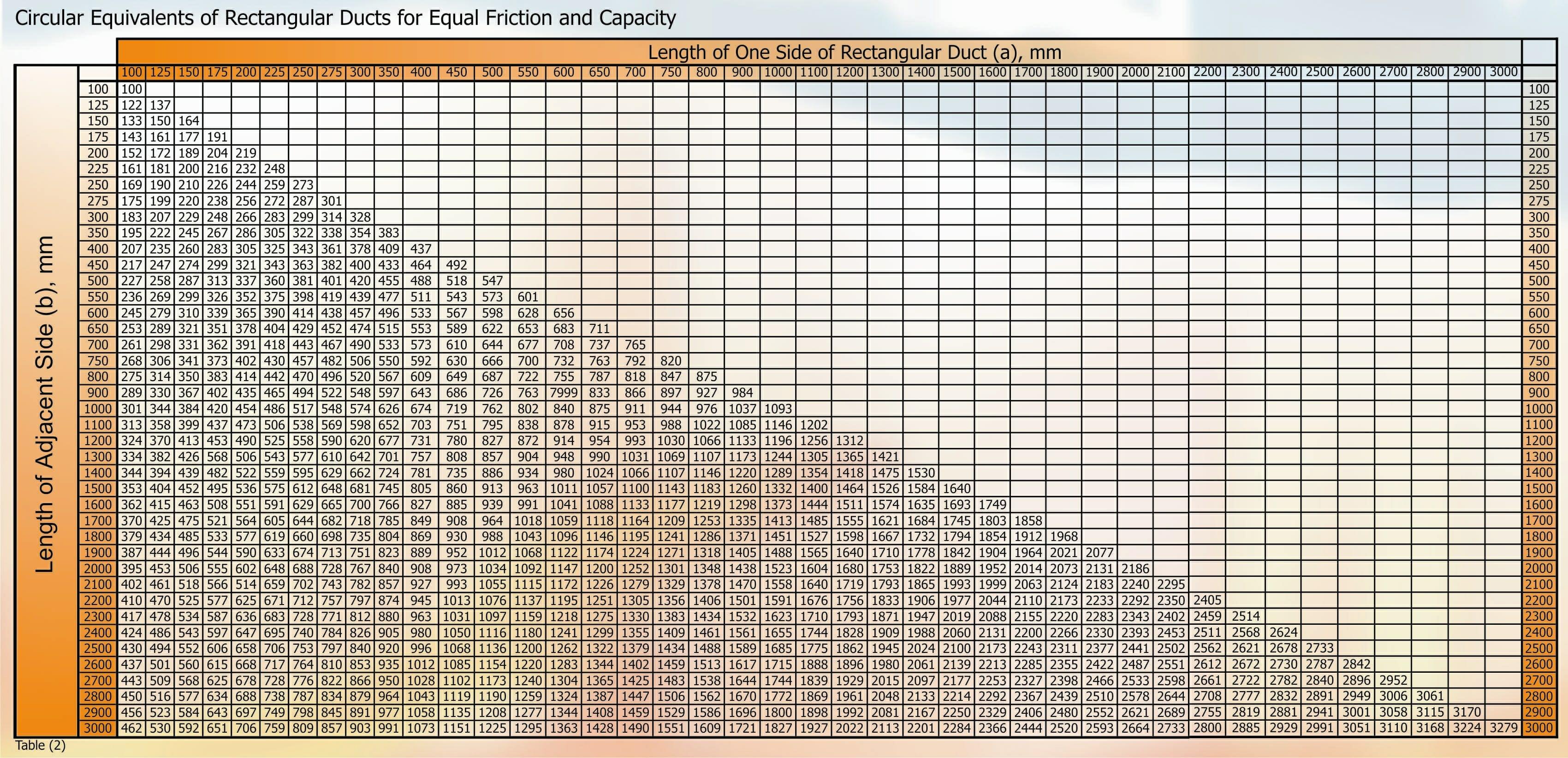
Most of the major air conditioning manufacturers can provide charts giving the equivalent hydraulic diameters for rectangular duct sections. The chart shown in this article (Table 2) is a print out from a spread sheet using the above formula.
Additional information that has to be determined are the pressure drop required by the discharge diffusers in order to achieve the required distribution characteristics. This figure will have to be added to the duct pressure loss together with losses from all components, such as inlet louvres, filters, pre-heaters etc. fitted before the fan and between the fan discharge and diffusers.
Velocity Reduction
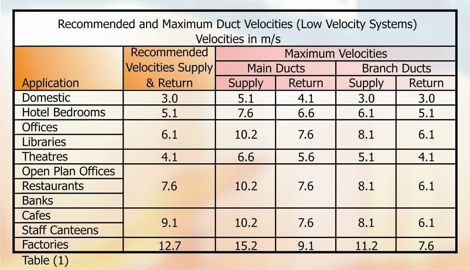
This method of calculation is based on setting the initial velocity at the beginning of the main duct, in accordance with the recommended velocity for the given application as shown in Table 1. This velocity is then reduced by an arbitrary amount after each junction. The reduction of velocity at each junction will be influenced by the number of junctions from the main duct. The object is to maintain a velocity greater than the recommenced velocity for a branch duct at the last duct junction.
Having determined the velocity, it is then a simple matter to calculate the required cross sectional area require to achieve this figure using the formula;
Velocity (V) in m/s
V = Q/A
Where Q = Air Volume m³/s and A = cross sectional area of duct m² .
Therefore the area A = Q/V;
Thus & so
If rectangular ducts are to be used then enter the chart giving Circular Equivalents of rectangular ducts by converting D from m to D in mm. Then select the desired length of one side in mm and move horizontally until the dimension of the diameter is found. If necessary, interpolate between rows or columns.
Calculate the total pressure drop of the longest run, taking into consideration all fittings in the run, (generally the longest run has the greatest pressure drop but a shorter run with a large number of fittings may have a greater pressure drop, therefore unless it’s obvious which run has the highest loss it will be prudent to undertake check calculations on other runs.) The highest pressure drop run is called the Index Run. This figure will be used to select the fan.
To minimise balancing of duct flows, a check calculation should be performed to establish the pressure loss in each of the branches, then duct dimensions adjusted to equalise the losses to ensure the correct pressure is available at each diffuser.
Return duct design should be undertaken in a similar manner with the highest velocity located nearest the exhaust fan or discharge outlet.
Equal Friction
As the name implies this method of design is based on all duct runs having the same friction loss. The starting velocity is selected using Table 1 – Maximum velocities. Using this figure in conjunction with the total volume of air to be supplied, enter Chart 2 or 2a. With the total volume of air expressed in litres per sec (l/s), move vertically along the volume line until it intersects with required angled velocity curve and at the intersection of these two lines, traverse horizontally to read the Fraction Loss in Pascal’s per metre (Pa/m). Note the name Fraction, not Friction. This because we are looking at the pressure loss per unit length.
All remaining duct selections will be at the same pressure loss established above. All that has to be done is to enter all subsequent air volumes on the “x” axis and read the velocity at the point of intersection with the pressure loss line. However care has to be taken to ensure that the velocities resulting from these readings do not exceed the maximum velocities recommended. If this does occur, then a lower starting velocity should be used.
The total length of each run must be calculated including the equivalent length of all fittings and this figure is then multiplied by the Fractional Pressure Loss to establish the total loss of the duct run. The fan is then selected to match the total loss figure.
Static Regain
A simplistic explanation of this method of calculation is to say that the object of this calculation is to ensure that the same pressure is available at each take off point by converting Velocity Head Pressure to Static Pressure, i.e. Static Regain. The conversion of velocity head takes place after each branch and is calculated to match the loss in the length of duct up to the next branch. With this method of calculation, the balancing of the system is made much easier and there can be cost savings resulting from the reduced need for balancing dampers.
In order to explain the Static Regain method of calculation fully, it is necessary to use an example and follow the calculation process, step by step. However in order to do this, a number of additional charts and tables will be required, but insufficient space is available to incorporate these charts in this months article. Therefore, the additional charts will be included in next months article and we will then continue with the explanation.
Constant Velocity
The constant velocity method of calculation is usually restricted to dust and fume extraction systems where the object is to entrain dust particles in the air stream. The velocity must be maintained at a sufficiently high level to carry the particles to a collector receptacle. The velocity is then reduced to a level which will no longer support or suspend the particles and they then simply drop out of the air stream for collection. See Table 5, Contaminant Transport Velocities and Table 5a Contaminant Capture Velocities in Part 2 next month.
With the above parameters established we can prepare to design the duct system. However, correct duct design requires the following information at various points in the design process:
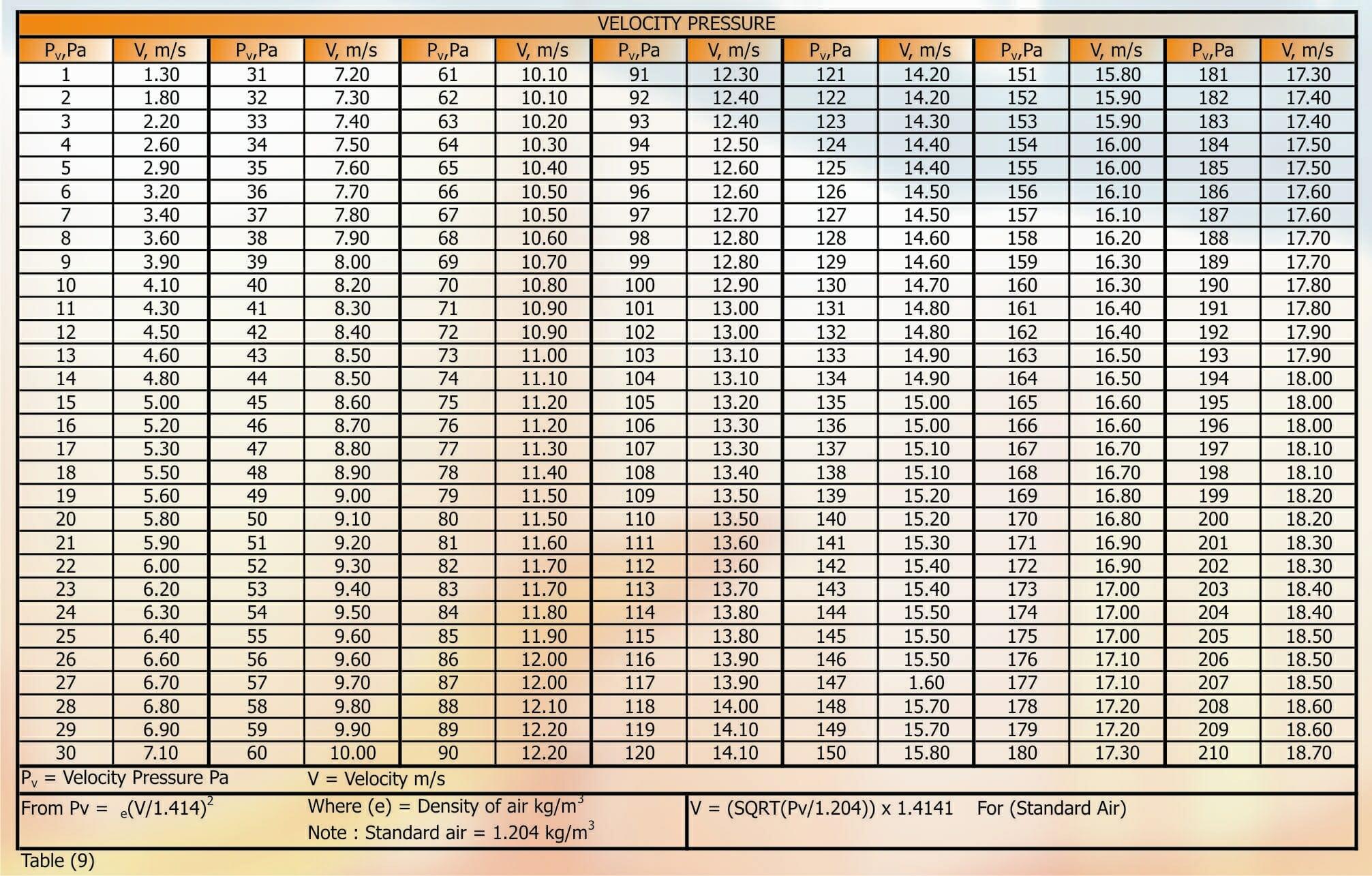
Velocity Pressure (Pv) in Pa (Pascals)
Where e = air density in kg/m³. (Standard air = 1.204 kg/m³ )
When working with Standard Air this formula can be reduced to:
To assist, a Velocity v Velocity Pressure table is shown below.
In order to arrive at the most efficient ductwork design, an iterative process is required. When starting the design, a number of arbitrary parameters are used to establish dimensions and pressure losses throughout the system. On completion of the duct layout, the calculated friction losses may show an excessive loss and the section of duct at the root of this can be identified. Therefore, an adjustment in sizes will be required which may result in the main duct and / or the branch duct dimensions and types of elbows and branches being altered. For example, from a cost aspect, splitters and turning vanes may have been omitted. However, the resultant friction losses could have shown that these cost savings are offset by increased cost of a larger fan assembly.
After the duct design has been altered the losses will have to be recalculated.
There are a number of computer duct design programs that can speed the process but not all programmes can optimise the design. Since it is the optimising process that is time consuming and determines the effectiveness of the installation, this feature should be sought after in any program you may consider purchasing.
The design velocity can be determined from Table 1. This table shows a number of different applications and the recommended velocities for each of them. The table differentiates between applications that have noise as the primary consideration and those that have duct resistance as the controlling factor.
DISCLAIMER: Whilst every effort is made to ensure absolute accuracy, Business Edge Ltd. will not accept any responsibility or liability for direct or indirect losses arising from the use of the data contained in this series of articles.