 Cassette Split Systems
 Safety Gloves
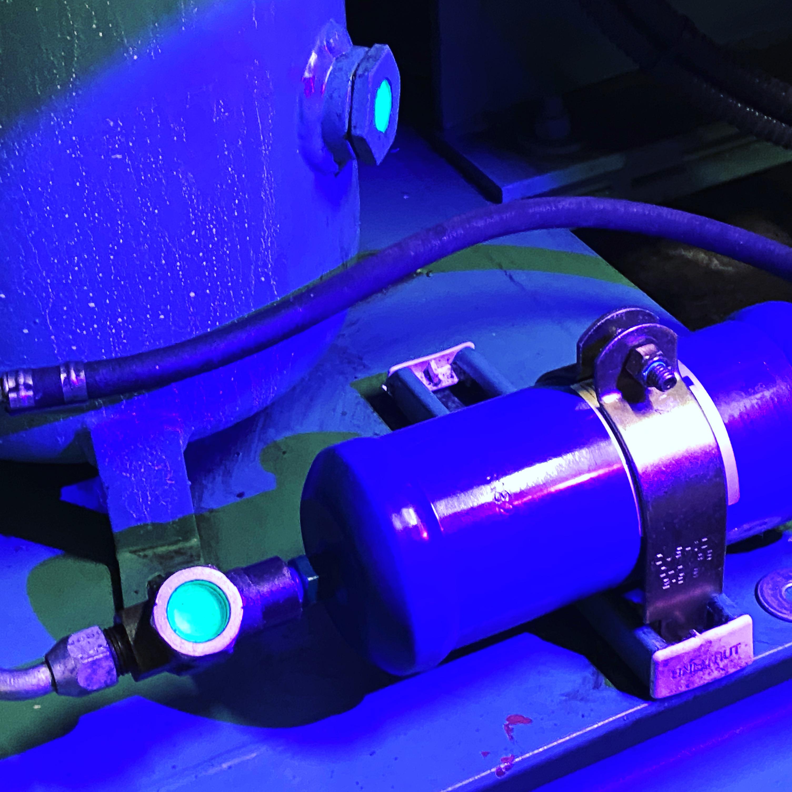 UV Leak Detection
 Condensate Drain Pipe
MASTERCLASS – AIR CONDITIONING TECHNOLOGY
Volume 38 – Duct Design
In the previous article the various methods used to calculate the pressure loss through ducts were briefly described. In this article we will follow a worked example using the Equal Friction Method of calculation.
Duct Design.
When commencing the duct design, the heat load in the various spaces will have been calculated either manually (or by using heat gain/loss calculation software – such as Quantum written by Business Edge Ltd – www.BusinessEdgeLtd.co.uk) and from this information the quantity of air and its condition will have been established using the methods described in previous articles. We therefore know how much conditioned air has to be circulated but do not know the required fan characteristics or how much energy is required to circulate the air.
The duct manufacturing standards are different for each category of duct system but it is quite common to combine categories of duct design in a single system. For example, a large office complex requiring very large volumes of air may use high velocity ductwork for the main runs and low velocity ductwork for the branch runs.
It is important to ensure that the appropriate duct manufacturing standard is used for each category of ductwork.
When designing ductwork numerous tables showing the either the pressure loss or the equivalent length of each fitting in the duct run have to be used and there are many sources for this information, ranging from the established reference manuals such as HVCA DW/143 / DW/144, CIBSE hand books or the ASHRAE Guide and Data Books. In addition, many major equipment manufacturers publish data in their own design manuals. Duct design, because of its use of tables and formulae lends itself to computer software programs which undoubtedly make life easier for the design engineer. However, these still require skill in their use by the engineer interpreting the information and converting this into an efficient and cost effective installation.
Engineers will, over a period of time, have found a source of tables and charts which have proven to be reliable and convenient to their style of working. In our worked example we will be using data published in ASHRAE and tables published in the Handbook of Air Conditioning System Design, published by The Carrier Air Conditioning Company. (For which we express our appreciation).
Step 1.
Study the conditioned spaces and locate the outlet diffusers and return air louvres. The location of these items must take into consideration:
- The number of air changes.
- Temperature gradients.
- Work patterns of the occupants.
Establish the required pressure drop for each of the outlet and inlet fittings necessary to achieve the design air pattern.
(The design and selection of diffuser and louvres is a topic in its own right and will be covered in the near future.)
Step 2.
Identify the route of the ductwork, noting the space available. Maximise the use of circular ductwork and when rectangular is used, endeavour to maintain the lowest practical aspect ratio’s for each of the runs.
Step 3.
Prepare a preliminary layout based on recommended velocities and ascertain if the duct sizes can be accommodated.
Step 4.
Calculate the duct losses. If the resultant calculations reveal excessive losses then adjust duct sizes. Alternatively, it may be possible to identify duct sections which can be reduced to improve the economics of the installation.
Step 5.
It may be necessary to repeat steps 3 and 4 a number of times before the optimum design is established.
Step 6.
Analyse the design for potential noise problems and incorporate the necessary fittings. Adjust calculations to take any additional pressure losses arising from the use of noise attenuators into account.
Step 7.
Prepare final manufacturing drawings.
Step 8.
Select fan with the necessary characteristics.
To place the above steps into context we will examine and calculate the characteristics of the duct layout shown see figure 1.

This scheme assumes that we have based the design on a low velocity system and from our preliminary layout the dimensions shown can be accommodated within the building.
The overall design parameters are as follows;
The application is an open plan office.
Total air volume flow rate = 2.25 m³/s
Main duct velocity = 7.6 m/s
The starting size of the main duct is established by table 1 (Master Class 37 recommended and maximum velocities).
Main duct size, circular area =Volume/velocity = 2.25/7.6 =0.296 m².
Therefore diameter = 0.614 m = 614 mm
Using table 2 (Master Class 37 circular equivalents of rectangular ducts) giving the equivalent rectangular duct dimensions we find that a duct with the long side of 800 mm and short size 400 mm has the equivalent diameter of 609 mm.
Since this duct has a diameter slightly less than was calculated, a check to find the actual velocity will show:
= 7.72 m/s which is only 0.12 m/s higher and acceptable.
On the basis of the known air volumes required in each branch duct and diffuser leg, we could approximate the sizes for all the ducts and following calculations, amend the duct sizes until we achieve the required result. However table 3 (Percent Section Area in Branches) allows us to speed up the process with much more accurate results.
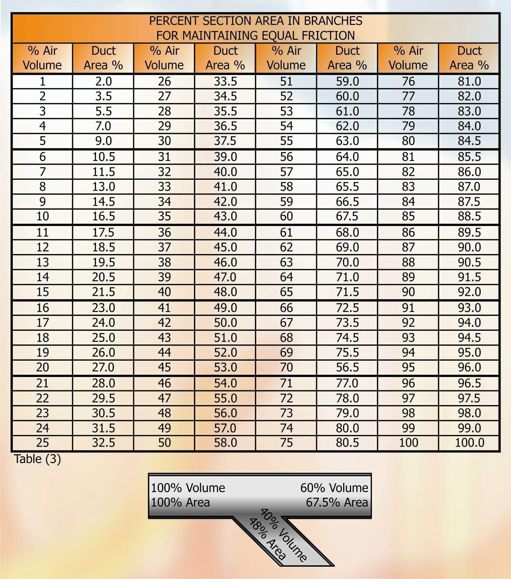
To use table (3) we must establish the percentage of air leaving the main duct at the branch. With this percentage we can then read the duct Circular Equivalent (referred to as Ce) as a percentage of the main ducts Ce area.
In figure 1: 750 l/s passes into the branch duct at (B);
Percentage of total volume entering branch =
From the table we read adjacent to 33% air volume that the duct area required is 41% of the Ce area of the main duct. Main ducts Ce area = 0.291 m²
Therefore branch duct Ce area = 0.291 x 0.41 = 0.119 m².
Volume of air in the next section of duct = 1500 l/s.
Expressed as a percentage of the total =
From the table we read 73.5% of main duct area required = 0.291 x 0.735 = 0.214 m². Ce area.
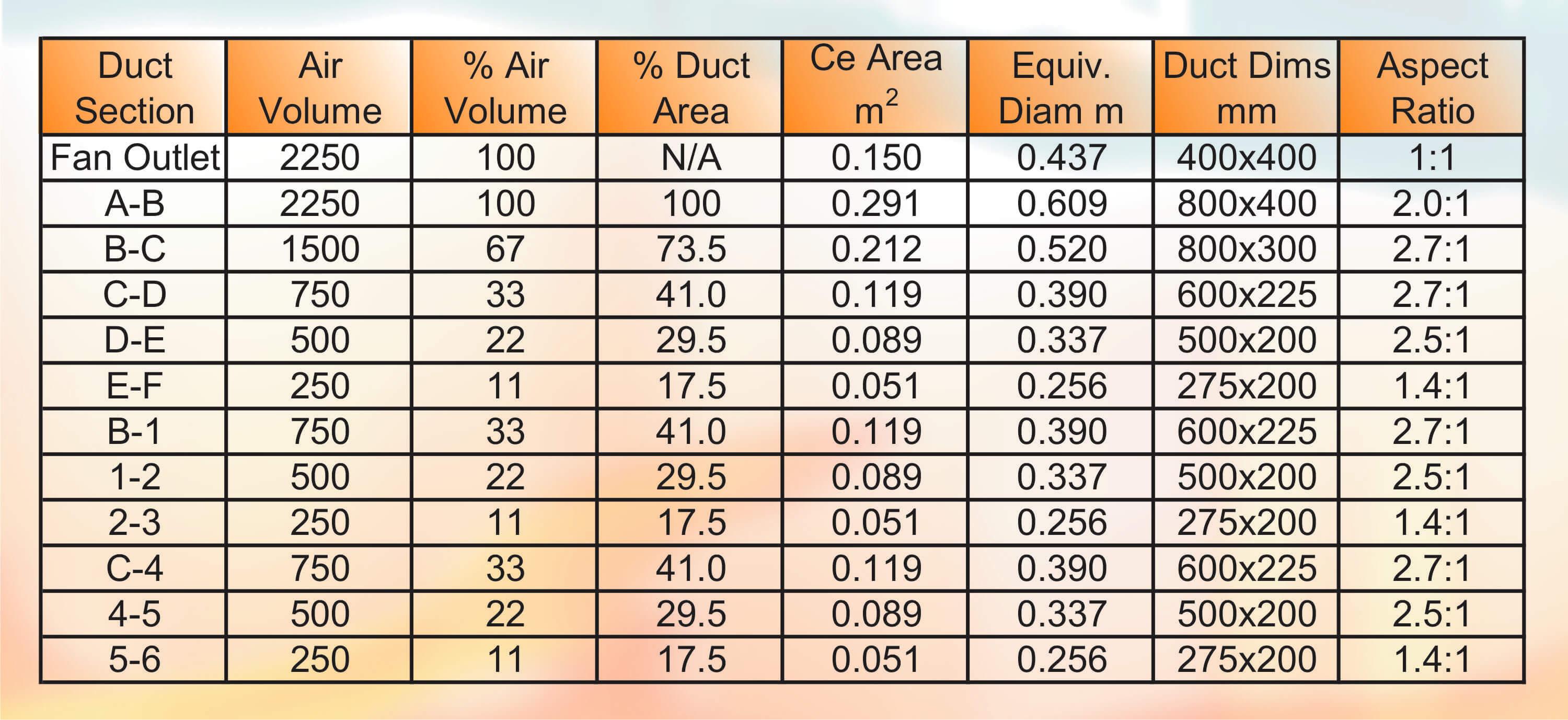
The exercise is repeated for all the ducts in the system and the following table is compiled.
Note: When using tables or charts calculations based on velocity e.g. Velocity pressure, then the actualvelocity must be established by dividing the volume by the actual cross section area of the fitting, not the equivalent area. Calculations to arrive at the friction loss through a fitting must always use the equivalent area.
Duct Sizing
Working in the direction away from the fan; the first duct fitting is the fan to duct transform section, marked on figure 1 as (i).
To obtain the local loss coefficient Co we enter the table (Plane Asymmetric Diffuser with Ductwork).
Here we must establish the Ce area ratio .
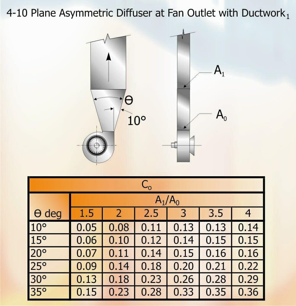
A1 = Ce cross sectional area of main duct = 0.291 m².
Ao = Ce area of fan outlet = 0.150 m².
Therefore the ratio will be .
The duct divergence angle is designed to be 20°.
The intersection of the x axis () and y axis (q °) for this fitting is:
Co = 0.1 (by interpolation).
The area of the fan outlet (Rectangular dimensions 400 mm x 400 mm) is 0.16 m2.
Therefore actual velocity will be = m/s.
Using either the Velocity Pressure table 9 (Master Class 37) or the formula we establish the velocity pressure (pv) = 119.1 Pa
Therefore pressure loss for Fan Transform = velocity pressure x fitting loss coefficient = 119.1 x 0.1 = 11.9 Pa.
The next fitting shown (ii) is a right angle mitred elbow with single thickness vanes. When calculating the pressure loss for this fitting, the key elements are the radius of the vanes r, the distance between vanes s and the length of the trailing edge of the vane L.
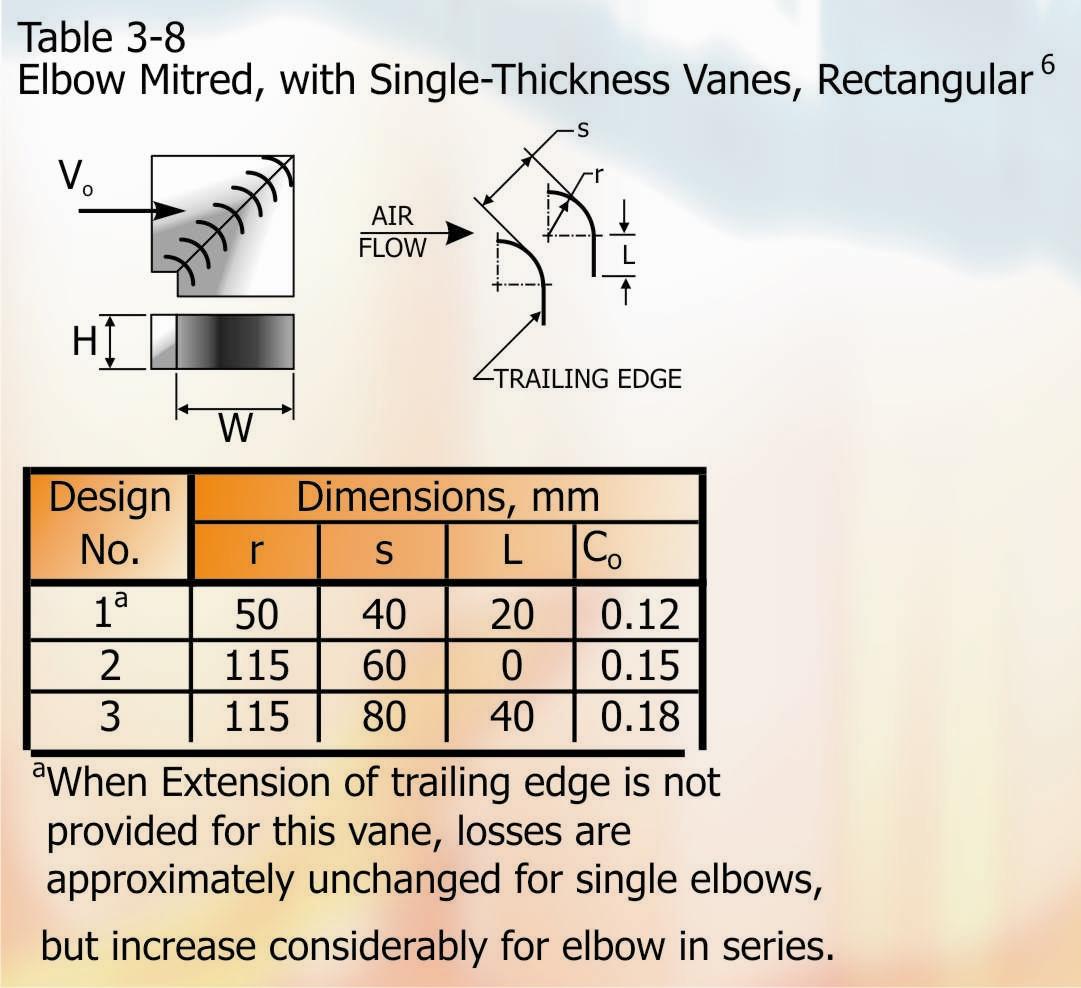
The radius and distance between vanes will be determined by the size of the elbow and its associated manufacturing cost. For this size of elbow we will use a radius of 115 mm set at 60 mm apart without any trailing extensions. For this design, the loss coefficient Co is 0.15. The velocity pressure for a duct 800 x 400 mm with an actual velocity of 7.03 m/s is 29.8 Pa. Therefore the loss through the elbow = 29.8 x 0.15 4.5 Pa.
Figure 1, shows that the next fitting in the main duct is a diverging “Y” branch fitting (iii).
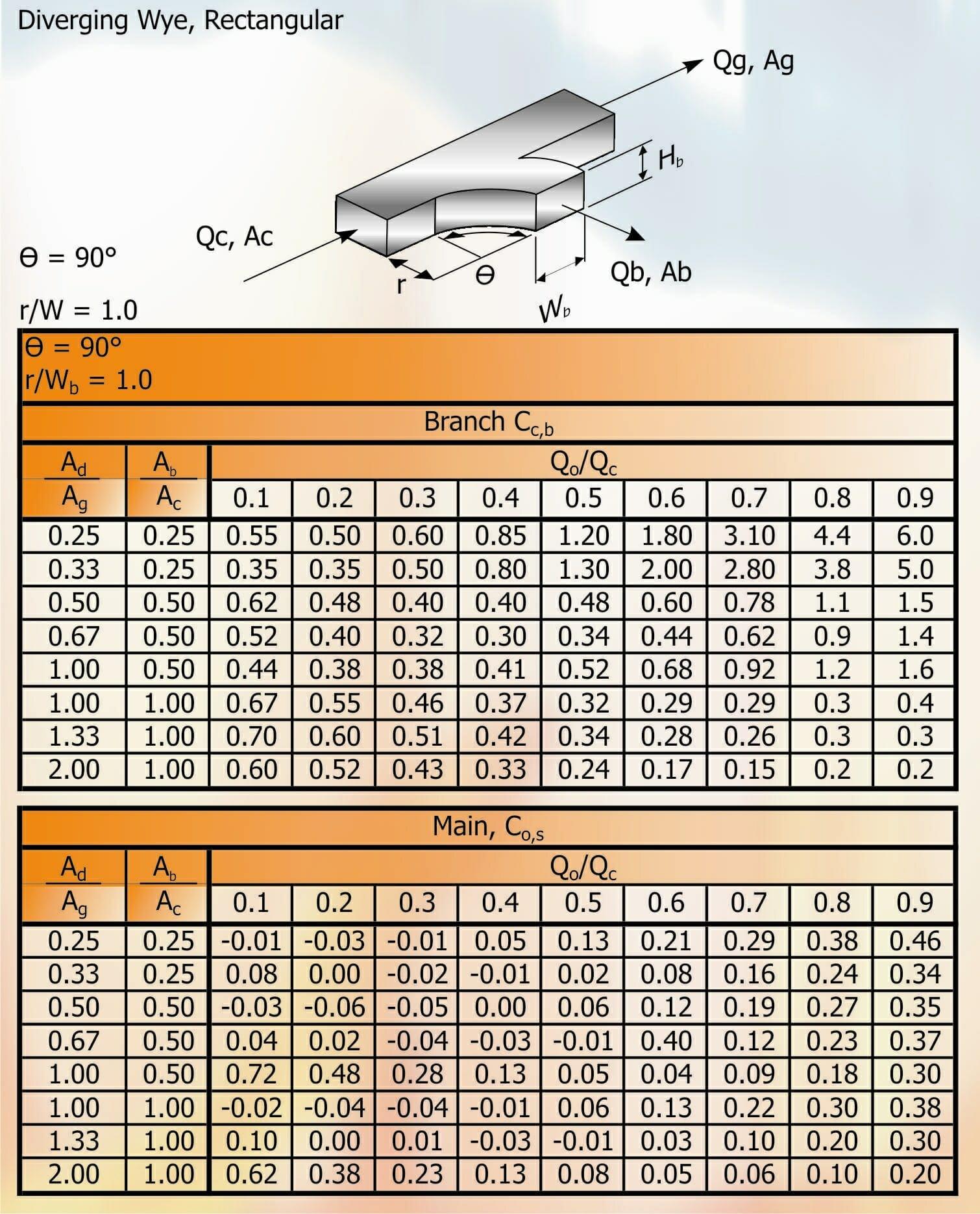
The calculation parameters are volume of air entering fitting (Qc), volume leaving at branch (Qb). Area at entry to fitting (Ac) and area of branch outlet (Ab) together with area of main outlet As. We also require the velocity pressure and since the duct section at Qc is the same as the previous fitting and the air volume is the same the velocity pressure will be 29.8 Pa.
Since we are concentrating on the losses in the main duct run we enter the table at = .
The loss coefficient ratio
The intersection of and = -0.04.
Then the loss or (gain) will be Pv x Cc = 29.8 x –0.04 = -1.192 Pa.
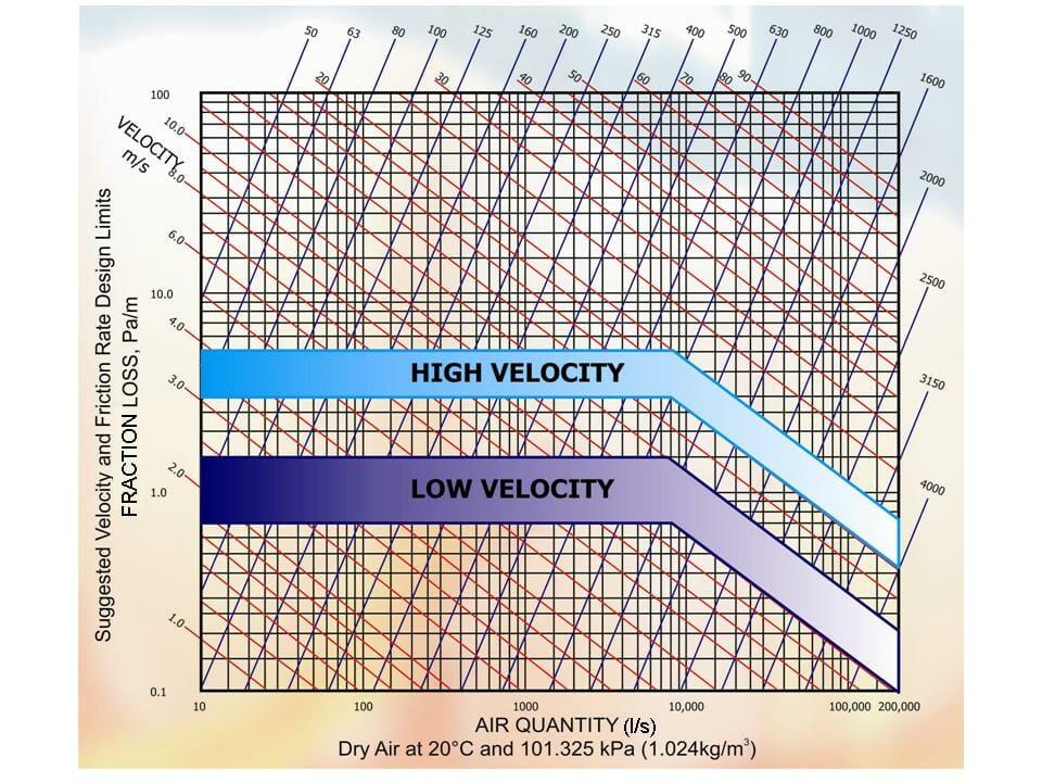
The total length of duct between fittings (A) and (B) is made up of ducts D1 and D2. If we enter Chart 5 at the air quantity and rise vertically until the line intersects with equivalent duct diameter 609 mm we establish the fraction loss is 0.8 Pa/m. Therefor the losses through these ducts are;
D1 = 6 x 0.8 = 4.8 Pa. and D2 = 15 x 0.8 = 12.0 Pa.
Immediately after fitting (iii) we must reduce down to duct section D3 via a duct transition piece fitting (iv).
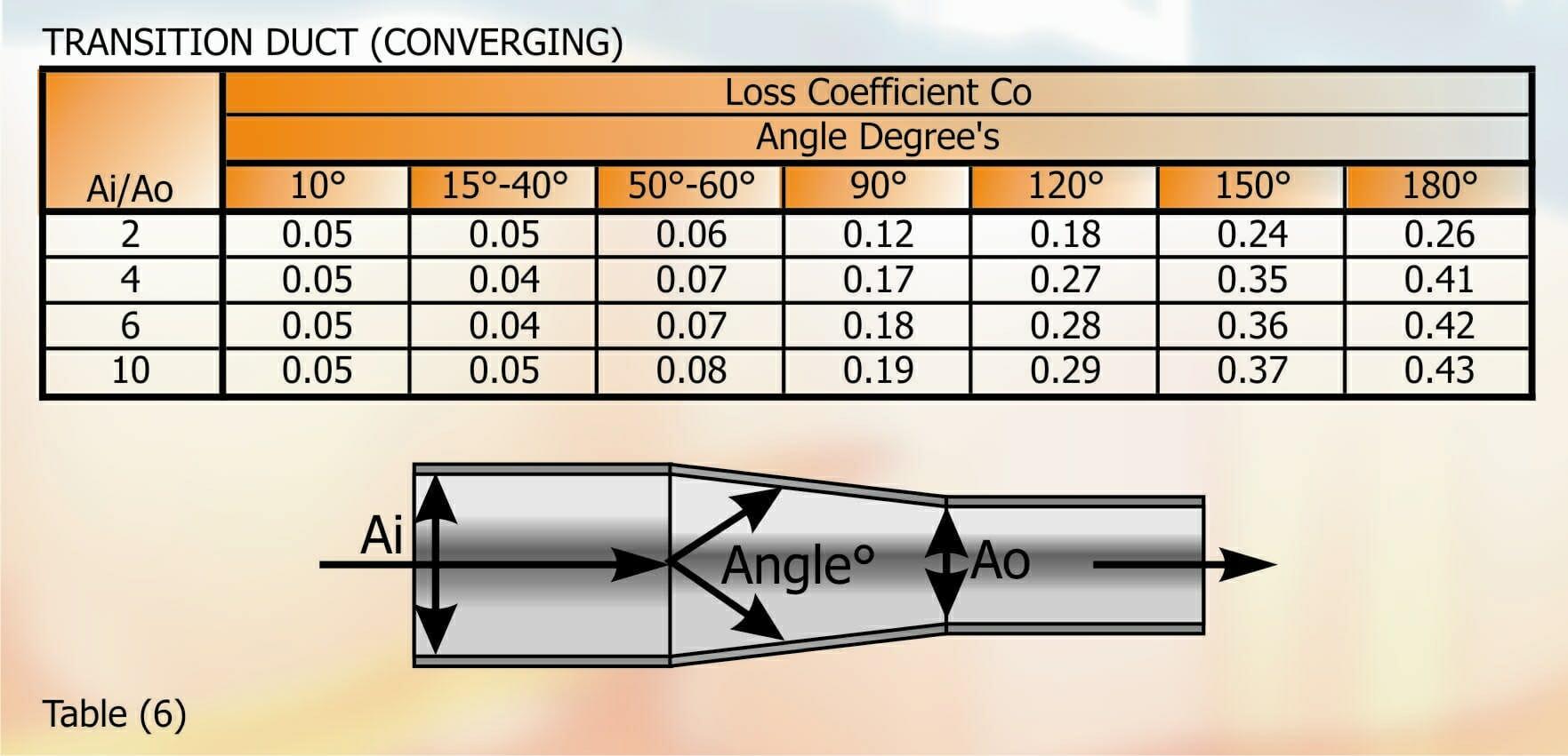
Table 6 is used in conjunction with Duct Sizing Table. We have to establish the inlet Ai to outlet Ao area ratios together with the angle of slope between inlet and outlet. We have decided the slope angle will be between 15° and 40°. The ratio Ai/Ao = 0.291/0.212 = 1.373 since this figure is less than two we look at the intersection of 2 on y axis and 15°- 40° on the x axis to read Co = 0.05. The velocity and velocity pressure are respectively;
m/s and from the Velocity Pressure table Pv = 23.5 Pa.
Therefore the loss will be 23.5 x 0.05 = 1.2 Pa.
We now come to fitting (v) a diverging “T”. To establish the loss coefficient for this fitting we have to calculate the velocity ratio of the air entering the “T” and the velocity of the air leaving the “T”. From figure 1 we see that the “T” has a section 800 mm x 300 mm and the volume entering is 1500 l/s. This equates to a velocity of 6.25 m/s and a velocity pressure of 23.5 Pa. The volume of air leaving the “T” is 750 l/s giving a velocity of 3.125, velocity ratio = From the Chart 2 we find Cc = 0.09. Pressure loss = 23.5 x 0.09 = 2.12 Pa.
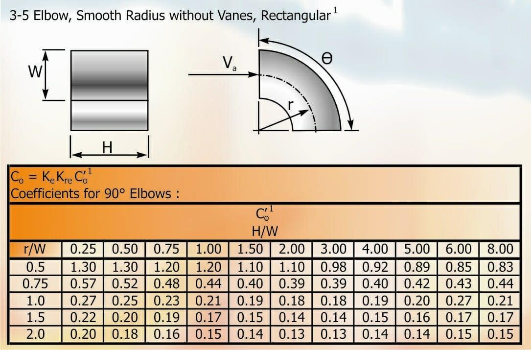
Following the “T” we have a transformation piece (vi) and we have already shown how to calculate the loss through this type of fitting, so we now examine fitting (vii) which is an elbow without vanes in the main duct run. The variables used in calculating the losses are the ratio of the centre line radius r divided by the width W of the duct: .
We need the height ratio: . The intersection of and reads C’o = 0.18.
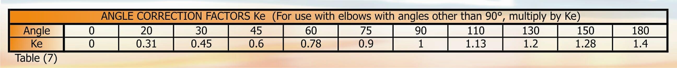
However the loss coefficient With Ke being a correction factor for angles other than 90°(See table 7) therefore in this instance Ke = 1. KRe is the correction factor based on Reynolds number for standard air (66.3).
D = the circular equivalent diameter in mm
Vo is the velocity in m/s
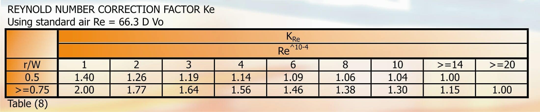
Re x 10-4 Therefore 143765 x 10-4 = 14.3765
Table 8 shows that if Re x 10-4 =>14 and if =>0.75 then KRe = 1.15.
Therefore Co = 1 x 1.15 x 0.18 = 0.21.
Diverging Y’s (viii) and (x) are calculated in the same way as (iii).
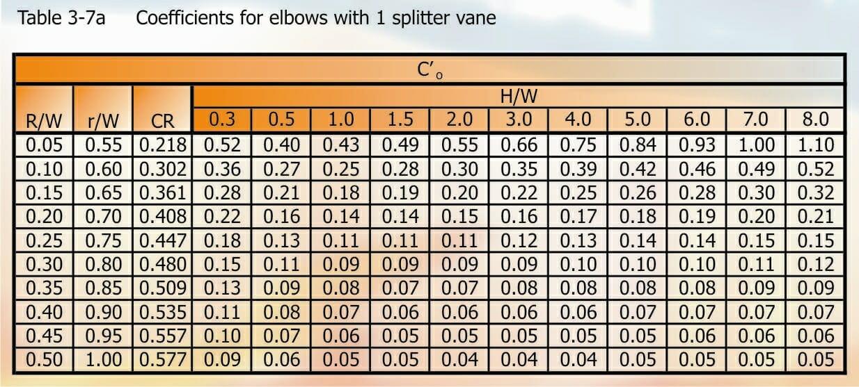
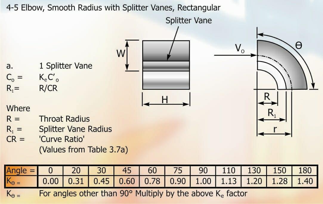
We now come to fitting (xii), a 90° radius bend containing a single turning vane. To establish Co we must identify the interim loss coefficient C’o.
C’o is a function of the radius or curve ratio and the ratio of the depth of the duct W and its cross sectional length H. The radius for this bend has been selected as 200 mm and the W dimension is also 200 mm the H dimension is 275 mm.
= = 1, = = 1.38.
The intersection of these two numbers shows C’o = 0.05.
Ke is found from Table 7.
Using the Angle 90° Ke = 1.
Since Co = Ke x C’o = 1 x 0.05 = 0.05.
The loss at this fitting is Pv x Co.
From Table 9 velocity pressure (Masterclass Part 37) using velocity 4.55 we interpolate
@ 4.50 = 12 & @ 4.60 = 13 thus 4.55 = 12.5 Pa.
To double check we calculate using formula
Therefore =12.46
Pv = 12.46 Pa.
Then loss at this elbow = 0.05 x 12.46 = 0.62 Pa.
The total loss on the index run of the duct is the sum of all losses. The fan selection will be based on this figure.
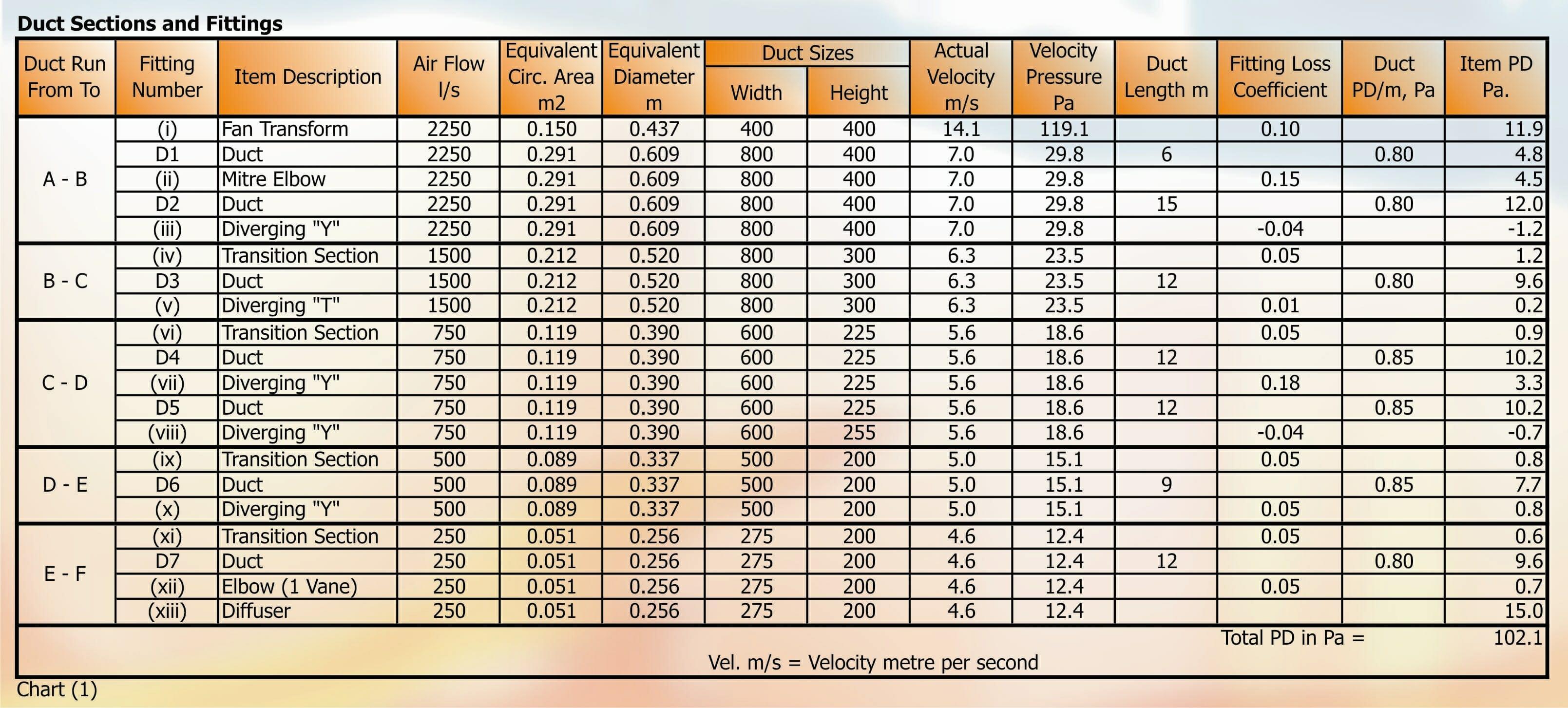
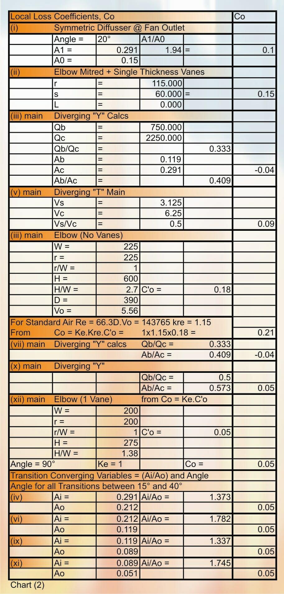
Chart (1) Shows a summary of the parameters used in arriving at the total loss for the index run.
Chart (2) Shows how the parameters used in Chart (1) were established.
DISCLAIMER: Whilst every effort is made to ensure absolute accuracy, Business Edge Ltd. will not accept any responsibility or liability for direct or indirect losses arising from the use of the data contained in this series of articles.